Import Libraries
import pandas as pd
import seaborn as sns
import matplotlib.pyplot as plt
from matplotlib.pyplot import figure
from itertools import combinations
from collections import Counter
Loading data
jan = pd.read_csv("Sales_January_2019.csv")
feb = pd.read_csv("Sales_February_2019.csv")
mar = pd.read_csv("Sales_March_2019.csv")
apr = pd.read_csv("Sales_April_2019.csv")
may = pd.read_csv("Sales_May_2019.csv")
jun = pd.read_csv("Sales_June_2019.csv")
jul = pd.read_csv("Sales_July_2019.csv")
aug = pd.read_csv("Sales_August_2019.csv")
sep = pd.read_csv("Sales_September_2019.csv")
octo = pd.read_csv("Sales_October_2019.csv")
nov = pd.read_csv("Sales_November_2019.csv")
dec = pd.read_csv("Sales_December_2019.csv")- First look
jan_head=jan.head()
jan_head.to_html()| Order ID | Product | Quantity Ordered | Price Each | Order Date | Purchase Address | |
|---|---|---|---|---|---|---|
| 0 | 141234 | iPhone | 1 | 700 | 01/22/19 21:25 | 944 Walnut St, Boston, MA 02215 |
| 1 | 141235 | Lightning Charging Cable | 1 | 14.95 | 01/28/19 14:15 | 185 Maple St, Portland, OR 97035 |
| 2 | 141236 | Wired Headphones | 2 | 11.99 | 01/17/19 13:33 | 538 Adams St, San Francisco, CA 94016 |
| 3 | 141237 | 27in FHD Monitor | 1 | 149.99 | 01/05/19 20:33 | 738 10th St, Los Angeles, CA 90001 |
| 4 | 141238 | Wired Headphones | 1 | 11.99 | 01/25/19 11:59 | 387 10th St, Austin, TX 73301 |
’
feb_head=feb.head()
feb_head.to_html()| Order ID | Product | Quantity Ordered | Price Each | Order Date | Purchase Address | |
|---|---|---|---|---|---|---|
| 0 | 150502 | iPhone | 1 | 700 | 02/18/19 01:35 | 866 Spruce St, Portland, ME 04101 |
| 1 | 150503 | AA Batteries (4-pack) | 1 | 3.84 | 02/13/19 07:24 | 18 13th St, San Francisco, CA 94016 |
| 2 | 150504 | 27in 4K Gaming Monitor | 1 | 389.99 | 02/18/19 09:46 | 52 6th St, New York City, NY 10001 |
| 3 | 150505 | Lightning Charging Cable | 1 | 14.95 | 02/02/19 16:47 | 129 Cherry St, Atlanta, GA 30301 |
| 4 | 150506 | AA Batteries (4-pack) | 2 | 3.84 | 02/28/19 20:32 | 548 Lincoln St, Seattle, WA 98101 |
’
mar_head=mar.head()
mar_head.to_html()| Order ID | Product | Quantity Ordered | Price Each | Order Date | Purchase Address | |
|---|---|---|---|---|---|---|
| 0 | 162009 | iPhone | 1 | 700 | 03/28/19 20:59 | 942 Church St, Austin, TX 73301 |
| 1 | 162009 | Lightning Charging Cable | 1 | 14.95 | 03/28/19 20:59 | 942 Church St, Austin, TX 73301 |
| 2 | 162009 | Wired Headphones | 2 | 11.99 | 03/28/19 20:59 | 942 Church St, Austin, TX 73301 |
| 3 | 162010 | Bose SoundSport Headphones | 1 | 99.99 | 03/17/19 05:39 | 261 10th St, San Francisco, CA 94016 |
| 4 | 162011 | 34in Ultrawide Monitor | 1 | 379.99 | 03/10/19 00:01 | 764 13th St, San Francisco, CA 94016 |
’
Merging all the dataset into one single file
- It’s looks like we have the same number of columns in each dataset. Let’s concatenate all of them
df = pd.concat([jan,feb,mar,apr,may,jun,jul,aug,sep,octo,nov,dec])
df_head = df.head()
df_head.to_html()| Order ID | Product | Quantity Ordered | Price Each | Order Date | Purchase Address | |
|---|---|---|---|---|---|---|
| 0 | 141234 | iPhone | 1 | 700 | 01/22/19 21:25 | 944 Walnut St, Boston, MA 02215 |
| 1 | 141235 | Lightning Charging Cable | 1 | 14.95 | 01/28/19 14:15 | 185 Maple St, Portland, OR 97035 |
| 2 | 141236 | Wired Headphones | 2 | 11.99 | 01/17/19 13:33 | 538 Adams St, San Francisco, CA 94016 |
| 3 | 141237 | 27in FHD Monitor | 1 | 149.99 | 01/05/19 20:33 | 738 10th St, Los Angeles, CA 90001 |
| 4 | 141238 | Wired Headphones | 1 | 11.99 | 01/25/19 11:59 | 387 10th St, Austin, TX 73301 |
’
- Let’s check the shape of it
df.shape #Looks good(186850, 6)Questions
- To perform our analysis in this dataset I’ll analyze and do the data cleaning within the questions that I want to answer.
Question 1: Whats was the best month for sales? How much was earned that month?
- We must check the dtypes of our data first:
df.info()<class 'pandas.core.frame.DataFrame'>
Int64Index: 186850 entries, 0 to 25116
Data columns (total 6 columns):
# Column Non-Null Count Dtype
--- ------ -------------- -----
0 Order ID 186305 non-null object
1 Product 186305 non-null object
2 Quantity Ordered 186305 non-null object
3 Price Each 186305 non-null object
4 Order Date 186305 non-null object
5 Purchase Address 186305 non-null object
dtypes: object(6)
memory usage: 10.0+ MB- We’ll collect the first 2 characters of the column “Order Date” but first we need to transform this column to string type
df['Order Date']=df['Order Date'].astype('string')- Now, we can see that the column “Order Date” changed to “string”
df.info()<class 'pandas.core.frame.DataFrame'>
Int64Index: 186850 entries, 0 to 25116
Data columns (total 6 columns):
# Column Non-Null Count Dtype
--- ------ -------------- -----
0 Order ID 186305 non-null object
1 Product 186305 non-null object
2 Quantity Ordered 186305 non-null object
3 Price Each 186305 non-null object
4 Order Date 186305 non-null string
5 Purchase Address 186305 non-null object
dtypes: object(5), string(1)
memory usage: 10.0+ MBdf["Order Date"]=df["Order Date"].str.replace("'","")
df["Order Date"]=df["Order Date"].str.replace("b","")- Creating a column named “Month”
df["Month"]=df["Order Date"].str[:2]- Creating a dictionary to replace the month numbers’s to the respective month
month_dict = {"01":"January","02":"February","03":"March","04":"April","05":"May","06":"June","07":"July",
"08":"August","09":"September","10":"October","11":"November","12":"December"}df["Month"]=df["Month"].replace(month_dict)- Modify the data type to numeric
df["Price Each"]=pd.to_numeric(df["Price Each"],errors='coerce')
df["Quantity Ordered"]=pd.to_numeric(df["Quantity Ordered"],errors='coerce')- Dropping the missing values in our dataset
df=df.dropna()- Creating new column that corresponds to the total sales
df["Total_Sales"] = df["Price Each"]*df["Quantity Ordered"]
df_head = df.head()
df_head.to_html()| Order ID | Product | Quantity Ordered | Price Each | Order Date | Purchase Address | Month | Total_Sales | |
|---|---|---|---|---|---|---|---|---|
| 0 | 141234 | iPhone | 1.0 | 700.00 | 01/22/19 21:25 | 944 Walnut St, Boston, MA 02215 | January | 700.00 |
| 1 | 141235 | Lightning Charging Cable | 1.0 | 14.95 | 01/28/19 14:15 | 185 Maple St, Portland, OR 97035 | January | 14.95 |
| 2 | 141236 | Wired Headphones | 2.0 | 11.99 | 01/17/19 13:33 | 538 Adams St, San Francisco, CA 94016 | January | 23.98 |
| 3 | 141237 | 27in FHD Monitor | 1.0 | 149.99 | 01/05/19 20:33 | 738 10th St, Los Angeles, CA 90001 | January | 149.99 |
| 4 | 141238 | Wired Headphones | 1.0 | 11.99 | 01/25/19 11:59 | 387 10th St, Austin, TX 73301 | January | 11.99 |
’
- Creating a new variable to assign the month grouped
best_month=df.groupby(["Month"]).sum()
best_month.reset_index(inplace=True)
best_month
Month Quantity Ordered Price Each Total_Sales
0 April 20558.0 3367671.02 3390670.24
1 August 13448.0 2230345.42 2244467.88
2 December 28114.0 4588415.41 4613443.34
3 February 13449.0 2188884.72 2202022.42
4 January 10903.0 1811768.38 1822256.73
5 July 16072.0 2632539.56 2647775.76
6 June 15253.0 2562025.61 2577802.26
7 March 17005.0 2791207.83 2807100.38
8 May 18667.0 3135125.13 3152606.75
9 November 19798.0 3180600.68 3199603.20
10 October 22703.0 3715554.83 3736726.88
11 September 13109.0 2084992.09 2097560.13- Ploting the data using seaborn
sns.barplot(x="Total_Sales", y="Month", data=best_month);
plt.show()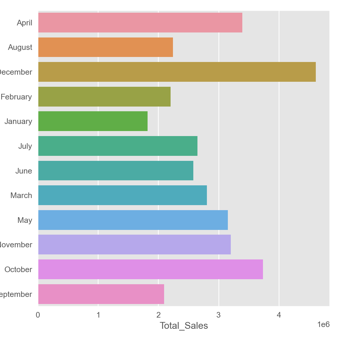
- December was the best month for sales. The total earned this month was $4.613.443,34.
Question 2: What city had the highest number of sales?
- Changing the datatype on the column “Purchase Address”
df["Purchase Address"]=df["Purchase Address"].astype('string')- Creating a new variable thats contains the city code
city=df["Purchase Address"].str.split(pat=",",expand=True)- Creating a new colunm to assign the values from the cities
df["City"]=city[1]- Let´s check how our df looks like now
df_head = df.head()
df_head.to_html()| Order ID | Product | Quantity Ordered | Price Each | Order Date | Purchase Address | Month | Total_Sales | City | |
|---|---|---|---|---|---|---|---|---|---|
| 0 | 141234 | iPhone | 1.0 | 700.00 | 01/22/19 21:25 | 944 Walnut St, Boston, MA 02215 | January | 700.00 | Boston |
| 1 | 141235 | Lightning Charging Cable | 1.0 | 14.95 | 01/28/19 14:15 | 185 Maple St, Portland, OR 97035 | January | 14.95 | Portland |
| 2 | 141236 | Wired Headphones | 2.0 | 11.99 | 01/17/19 13:33 | 538 Adams St, San Francisco, CA 94016 | January | 23.98 | San Francisco |
| 3 | 141237 | 27in FHD Monitor | 1.0 | 149.99 | 01/05/19 20:33 | 738 10th St, Los Angeles, CA 90001 | January | 149.99 | Los Angeles |
| 4 | 141238 | Wired Headphones | 1.0 | 11.99 | 01/25/19 11:59 | 387 10th St, Austin, TX 73301 | January | 11.99 | Austin |
’
- Creating a new variable that contains info for cities grouped
best_city=df.groupby(["City"]).sum()
best_city.reset_index(inplace=True)- Plotting the data
sns.barplot(x="Total_Sales", y="City", data=best_city);
plt.show()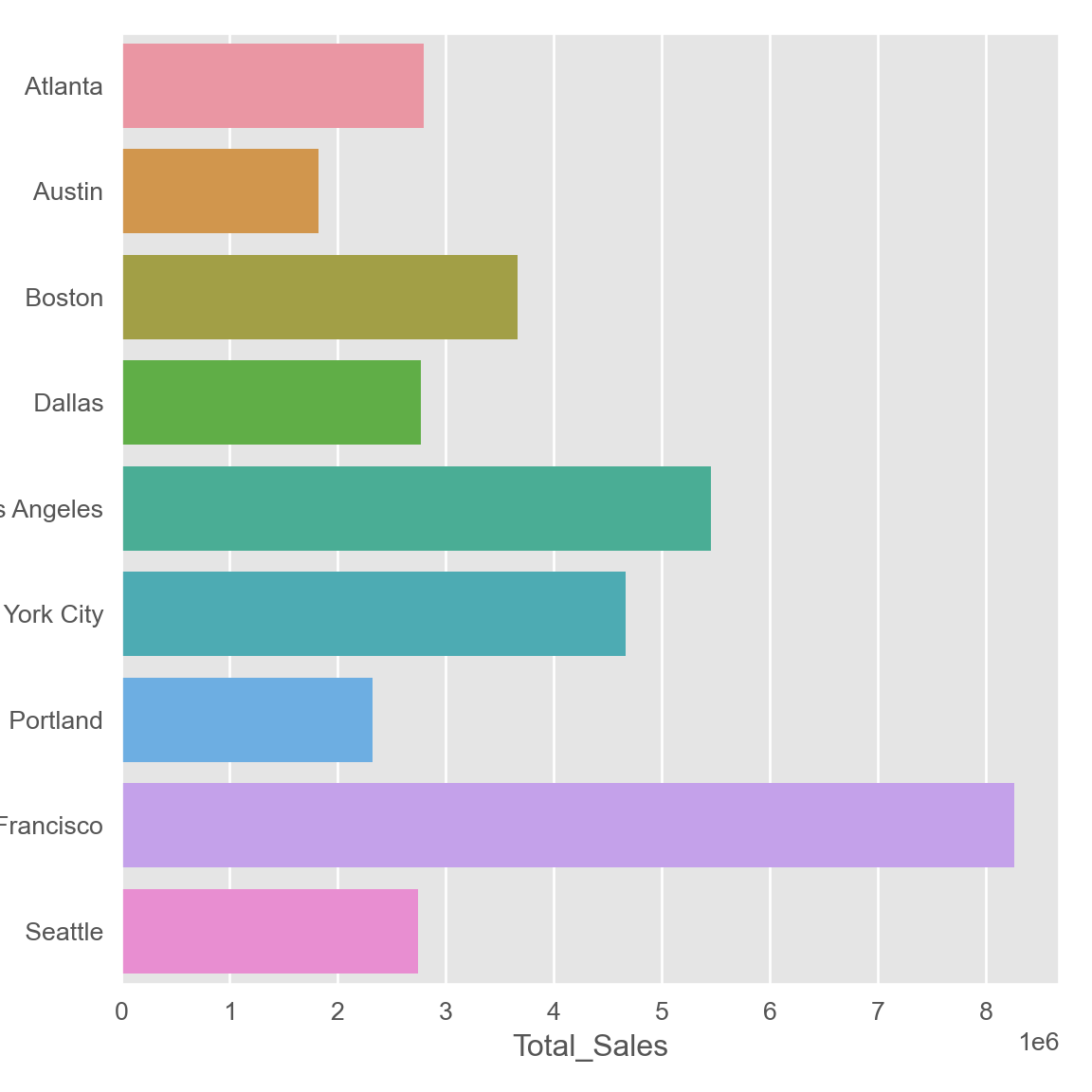
- The city which had the highest number of sales was San Francisco
Question 3: What time we should display the advertisements to maxime the likelihood of customer’s buying products?
- Changing the datetype to datetime to be able to extract the hour
df["Order Date"]=pd.to_datetime(df["Order Date"])
df["Hour"]=df["Order Date"].dt.hour- Creating a new variable the contains the info about hour grouped
hour=df.groupby("Hour").sum()
hour.reset_index(inplace=True)- Plotting using seaborn
sns.lineplot(data=hour, x="Hour", y="Total_Sales");
plt.xticks(hour["Hour"]);
plt.grid();
plt.show()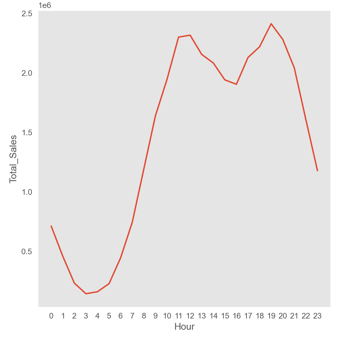
- The best time to display the advertisements is 19h (7 pm). My assumption that this occurs because it when people have already came back from work and they are having dinner at this moment, watching TV.
Question 4: What products are most often sold together?
- The products are sold together when they have the same order ID, therefore we need only the row that have the same number for Order ID, and we’ll assign it to a new dataframe
products=df[df["Order ID"].duplicated(keep=False)]
products_head=products.head()
products_head.to_html()| Order ID | Product | Quantity Ordered | Price Each | Order Date | Purchase Address | Month | Total_Sales | City | Hour | |
|---|---|---|---|---|---|---|---|---|---|---|
| 41 | 141275 | USB-C Charging Cable | 1.0 | 11.95 | 2019-01-07 16:06:00 | 610 Walnut St, Austin, TX 73301 | January | 11.95 | Austin | 16 |
| 42 | 141275 | Wired Headphones | 1.0 | 11.99 | 2019-01-07 16:06:00 | 610 Walnut St, Austin, TX 73301 | January | 11.99 | Austin | 16 |
| 57 | 141290 | Apple Airpods Headphones | 1.0 | 150.00 | 2019-01-02 08:25:00 | 4 1st St, Los Angeles, CA 90001 | January | 150.00 | Los Angeles | 8 |
| 58 | 141290 | AA Batteries (4-pack) | 3.0 | 3.84 | 2019-01-02 08:25:00 | 4 1st St, Los Angeles, CA 90001 | January | 11.52 | Los Angeles | 8 |
| 133 | 141365 | Vareebadd Phone | 1.0 | 400.00 | 2019-01-10 11:19:00 | 20 Dogwood St, New York City, NY 10001 | January | 400.00 | New York City | 11 |
’
- Now, we’ll join the produts which has the same order ID (grouped) and we’ll create a new column. After that, we’ll remove the duplicates
products["Grouped"]=products.groupby("Order ID")["Product"].transform(lambda x:', '.join(x))
products=products[["Order ID", "Grouped"]].drop_duplicates()- Here we’ll iterate the column Grouped to combine the values that has the same info in their row
count=Counter()
for row in products["Grouped"]:
    row_list=row.split(',')
    count.update(Counter(combinations(row_list,2)))

for key,value in count.most_common(1):
    print("Produts that are more often sold together are:", key)
Produts that are more often sold together are: ('iPhone', ' Lightning Charging Cable')Question 5: What product sold the most? Why do you think it sold the most?
- To find this answer we need to create a new variable and assign the product column grouped
sold_most1=df.groupby("Product")["Quantity Ordered"].sum()
sold_most=pd.DataFrame(data=sold_most1) # Creating a dataframe
sold_most.reset_index(inplace=True)
sold_most=sold_most.sort_values(by='Quantity Ordered',ascending=False)
sold_most.iloc[0] # Answer
Product AAA Batteries (4-pack)
Quantity Ordered 31017.0
Name: 5, dtype: object- Plotting in sns
sns.barplot(x="Quantity Ordered",y="Product",data=sold_most,palette='rocket');
plt.show()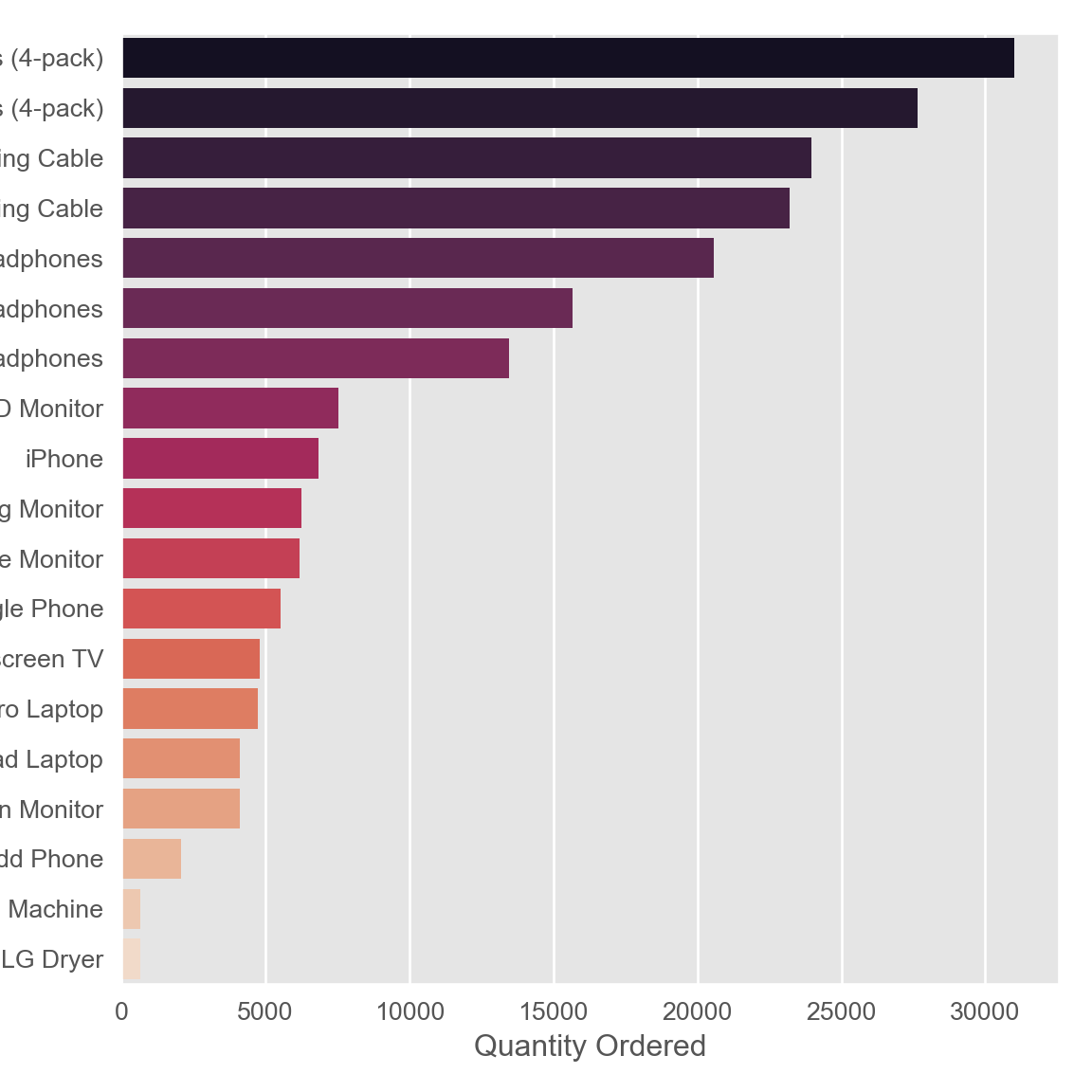
- Plotting in plt
plt.bar(sold_most["Product"],sold_most["Quantity Ordered"]);
plt.xticks(sold_most["Product"],rotation='vertical');
plt.show()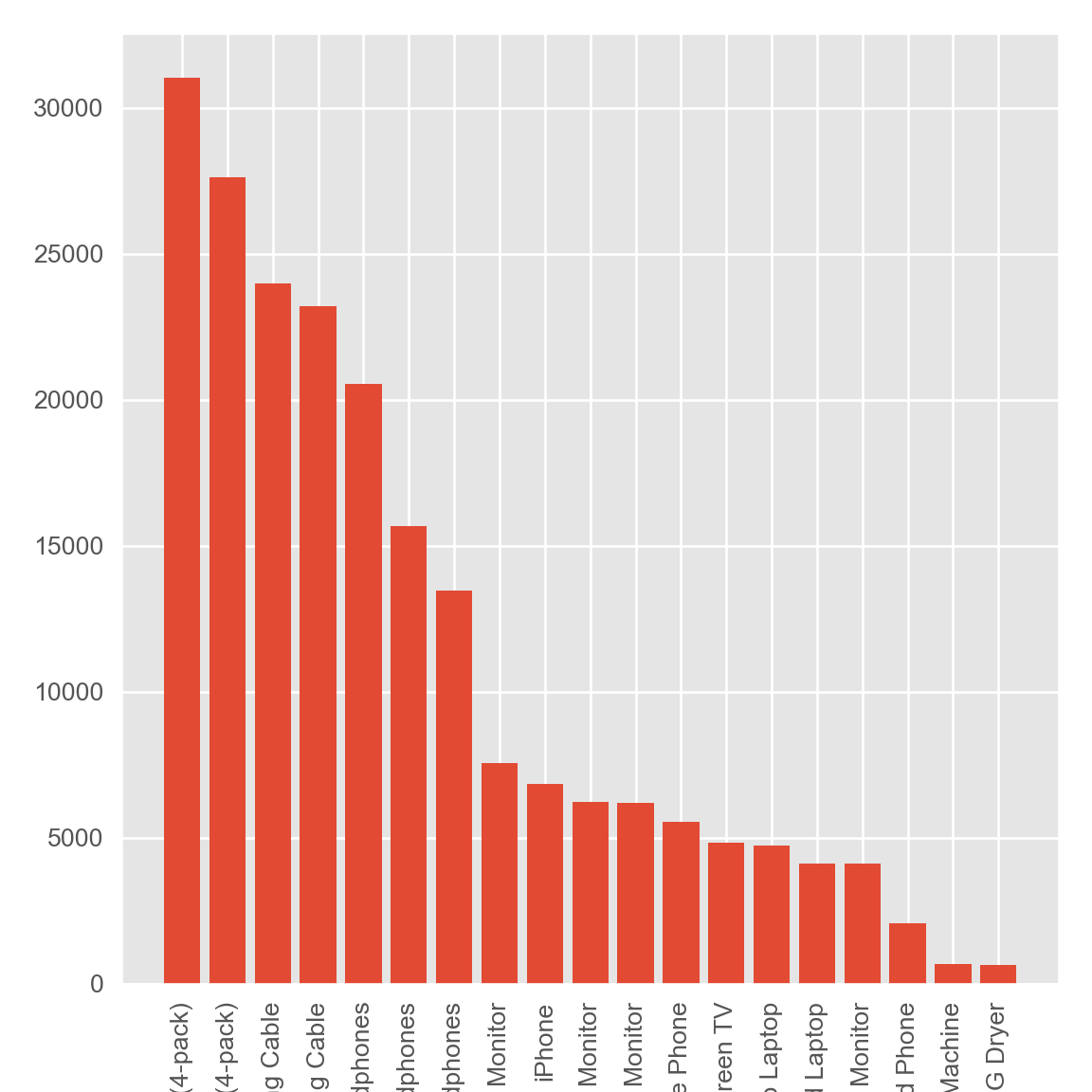
The AAA Batteries are the most sold product. My hypothesis it is because they are very cheap product. Lets confirm or not this statement
- Lets create a new dataframe with the mean values of the product prices
cheap1=df.groupby("Product")["Price Each"].mean()
cheap=pd.DataFrame(data=cheap1)
cheap.reset_index(inplace=True)
cheap
Product Price Each
0 20in Monitor 109.99
1 27in 4K Gaming Monitor 389.99
2 27in FHD Monitor 149.99
3 34in Ultrawide Monitor 379.99
4 AA Batteries (4-pack) 3.84
5 AAA Batteries (4-pack) 2.99
6 Apple Airpods Headphones 150.00
7 Bose SoundSport Headphones 99.99
8 Flatscreen TV 300.00
9 Google Phone 600.00
10 LG Dryer 600.00
11 LG Washing Machine 600.00
12 Lightning Charging Cable 14.95
13 Macbook Pro Laptop 1700.00
14 ThinkPad Laptop 999.99
15 USB-C Charging Cable 11.95
16 Vareebadd Phone 400.00
17 Wired Headphones 11.99
18 iPhone 700.00- Now, we’ll merge those both dataframe to create a visualization plot with both y axes
merg=pd.merge(sold_most,cheap,how='inner')- Plotting
sns.barplot(x="Product",y="Quantity Ordered",data=merg);
plt.xticks(rotation=90);
ax2 = plt.twinx();
sns.lineplot(x="Product",y="Price Each",data=merg, color="b", ax=ax2);
plt.show()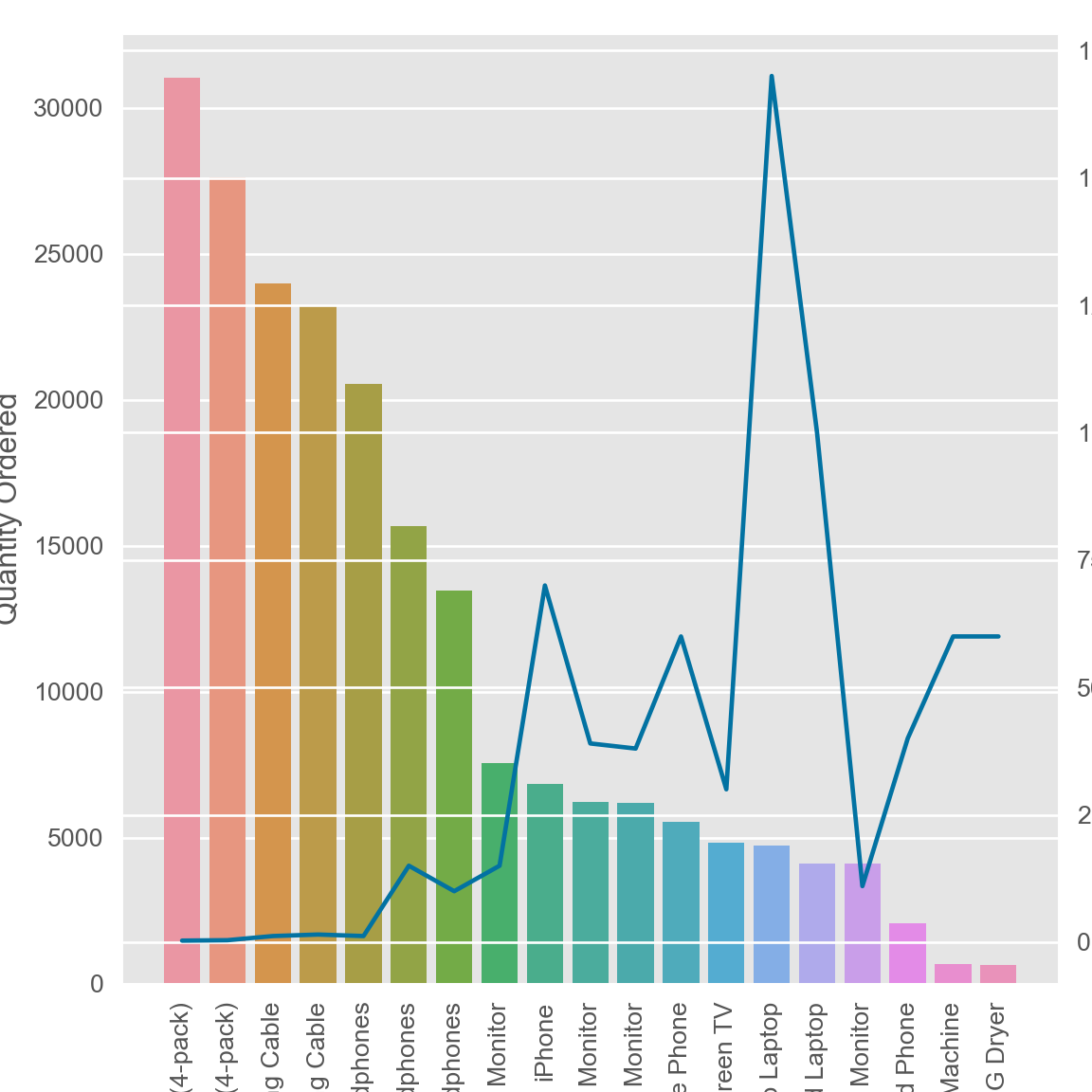
Conclusions
On this analysis we can conclude:
The best month of sales in December, most likely because of the holidays on the end of the year;
The city which had the highest number of sales is San Francisco;
The best time to display our marketing campaign is on 19h (7 pm);
The products that are more often sold together are IPhone and Lightning Charging Cable;
AAA batteries is the product that sold the most during the year, this happened because it is one of are chepaest products in store.