Importing Libraries
import numpy as np
import pandas as pd
import datetime
import matplotlib
import matplotlib.pyplot as plt
from matplotlib import colors
from matplotlib.colors import ListedColormap
import seaborn as sns
from sklearn import metrics
from sklearn.preprocessing import LabelEncoder
from sklearn.preprocessing import StandardScaler
from sklearn.decomposition import PCA
from sklearn.cluster import KMeans
from sklearn.cluster import AgglomerativeClustering
from yellowbrick.cluster import KElbowVisualizer
from mpl_toolkits.mplot3d import Axes3D
import warnings
import sys
if not sys.warnoptions:
    warnings.simplefilter("ignore")
np.random.seed(42)
Loading Data
data = pd.read_csv("marketing_campaign.csv", sep="\t")
print("Number of datapoints:", len(data))
Number of datapoints: 2240
df_head=data.head()
df_head.to_html()| ID | Year_Birth | Education | Marital_Status | Income | Kidhome | Teenhome | Dt_Customer | Recency | MntWines | MntFruits | MntMeatProducts | MntFishProducts | MntSweetProducts | MntGoldProds | NumDealsPurchases | NumWebPurchases | NumCatalogPurchases | NumStorePurchases | NumWebVisitsMonth | AcceptedCmp3 | AcceptedCmp4 | AcceptedCmp5 | AcceptedCmp1 | AcceptedCmp2 | Complain | Z_CostContact | Z_Revenue | Response | |
|---|---|---|---|---|---|---|---|---|---|---|---|---|---|---|---|---|---|---|---|---|---|---|---|---|---|---|---|---|---|
| 0 | 5524 | 1957 | Graduation | Single | 58138.0 | 0 | 0 | 04-09-2012 | 58 | 635 | 88 | 546 | 172 | 88 | 88 | 3 | 8 | 10 | 4 | 7 | 0 | 0 | 0 | 0 | 0 | 0 | 3 | 11 | 1 |
| 1 | 2174 | 1954 | Graduation | Single | 46344.0 | 1 | 1 | 08-03-2014 | 38 | 11 | 1 | 6 | 2 | 1 | 6 | 2 | 1 | 1 | 2 | 5 | 0 | 0 | 0 | 0 | 0 | 0 | 3 | 11 | 0 |
| 2 | 4141 | 1965 | Graduation | Together | 71613.0 | 0 | 0 | 21-08-2013 | 26 | 426 | 49 | 127 | 111 | 21 | 42 | 1 | 8 | 2 | 10 | 4 | 0 | 0 | 0 | 0 | 0 | 0 | 3 | 11 | 0 |
| 3 | 6182 | 1984 | Graduation | Together | 26646.0 | 1 | 0 | 10-02-2014 | 26 | 11 | 4 | 20 | 10 | 3 | 5 | 2 | 2 | 0 | 4 | 6 | 0 | 0 | 0 | 0 | 0 | 0 | 3 | 11 | 0 |
| 4 | 5324 | 1981 | PhD | Married | 58293.0 | 1 | 0 | 19-01-2014 | 94 | 173 | 43 | 118 | 46 | 27 | 15 | 5 | 5 | 3 | 6 | 5 | 0 | 0 | 0 | 0 | 0 | 0 | 3 | 11 | 0 |
’
Data Cleaning
In this section:
- Data Cleaning
- Feature Engineering
In order to, get a full grasp of what steps should I be taking to clean the dataset. Let us have a look at the information in data
#Information on features
data.info()
<class 'pandas.core.frame.DataFrame'>
RangeIndex: 2240 entries, 0 to 2239
Data columns (total 29 columns):
# Column Non-Null Count Dtype
--- ------ -------------- -----
0 ID 2240 non-null int64
1 Year_Birth 2240 non-null int64
2 Education 2240 non-null object
3 Marital_Status 2240 non-null object
4 Income 2216 non-null float64
5 Kidhome 2240 non-null int64
6 Teenhome 2240 non-null int64
7 Dt_Customer 2240 non-null object
8 Recency 2240 non-null int64
9 MntWines 2240 non-null int64
10 MntFruits 2240 non-null int64
11 MntMeatProducts 2240 non-null int64
12 MntFishProducts 2240 non-null int64
13 MntSweetProducts 2240 non-null int64
14 MntGoldProds 2240 non-null int64
15 NumDealsPurchases 2240 non-null int64
16 NumWebPurchases 2240 non-null int64
17 NumCatalogPurchases 2240 non-null int64
18 NumStorePurchases 2240 non-null int64
19 NumWebVisitsMonth 2240 non-null int64
20 AcceptedCmp3 2240 non-null int64
21 AcceptedCmp4 2240 non-null int64
22 AcceptedCmp5 2240 non-null int64
23 AcceptedCmp1 2240 non-null int64
24 AcceptedCmp2 2240 non-null int64
25 Complain 2240 non-null int64
26 Z_CostContact 2240 non-null int64
27 Z_Revenue 2240 non-null int64
28 Response 2240 non-null int64
dtypes: float64(1), int64(25), object(3)
memory usage: 507.6+ KBFrom the above output, we can conclude and note that:
- There are missing values in income
- Dt_Customer that indicates the date a customer joined the database is not parsed as DateTime
- There are some categorical features in our data frame; as there are some features in dtype: object). So we will need to encode them into numeric forms later.
First of all, for the missing values, I am simply going to drop the rows that have missing income values.
#To remove the NA values
data = data.dropna()
print("The total number of data-points after removing the rows with missing values are:", len(data))
The total number of data-points after removing the rows with missing values are: 2216In the next step, I am going to create a feature out of “Dt_Customer” that indicates the number of days a customer is registered in the firm’s database. However, in order to keep it simple, I am taking this value relative to the most recent customer in the record.
Thus to get the values I must check the newest and oldest recorded dates.
data["Dt_Customer"] = pd.to_datetime(data["Dt_Customer"])
dates = []
for i in data["Dt_Customer"]:
    i = i.date()
    dates.append(i)
#Dates of the newest and oldest recorded customer
print("The newest customer's enrolment date in therecords:",max(dates))
The newest customer's enrolment date in therecords: 2014-12-06print("The oldest customer's enrolment date in the records:",min(dates))The oldest customer's enrolment date in the records: 2012-01-08Creating a feature (“Customer_For”) of the number of days the customers started to shop in the store relative to the last recorded date
#Created a feature "Customer_For"
days = []
d1 = max(dates) #taking it to be the newest customer
for i in dates:
    delta = d1 - i
    days.append(delta)
data["Customer_For"] = days
data["Customer_For"] = pd.to_numeric(data["Customer_For"], errors="coerce")
Now we will be exploring the unique values in the categorical features to get a clear idea of the data.
print("Total categories in the feature Marital_Status:\n", data["Marital_Status"].value_counts(), "\n")Total categories in the feature Marital_Status:
Married 857
Together 573
Single 471
Divorced 232
Widow 76
Alone 3
Absurd 2
YOLO 2
Name: Marital_Status, dtype: int64 print("Total categories in the feature Education:\n", data["Education"].value_counts())Total categories in the feature Education:
Graduation 1116
PhD 481
Master 365
2n Cycle 200
Basic 54
Name: Education, dtype: int64In the next bit, I will be performing the following steps to engineer some new features:
- Extract the “Age” of a customer by the “Year_Birth” indicating the birth year of the respective person.
- Create another feature “Spent” indicating the total amount spent by the customer in various categories over the span of two years.
- Create another feature “Living_With” out of “Marital_Status” to extract the living situation of couples.
- Create a feature “Children” to indicate total children in a household that is, kids and teenagers.
- To get further clarity of household, Creating feature indicating “Family_Size”
- Create a feature “Is_Parent” to indicate parenthood status
- Lastly, I will create three categories in the “Education” by simplifying its value counts.
- Dropping some of the redundant features
#Feature Engineering
#Age of customer today
data["Age"] = 2021-data["Year_Birth"]

#Total spendings on various items
data["Spent"] = data["MntWines"]+ data["MntFruits"]+ data["MntMeatProducts"]+ data["MntFishProducts"]+ data["MntSweetProducts"]+ data["MntGoldProds"]

#Deriving living situation by marital status"Alone"
data["Living_With"]=data["Marital_Status"].replace({"Married":"Partner", "Together":"Partner", "Absurd":"Alone", "Widow":"Alone", "YOLO":"Alone", "Divorced":"Alone", "Single":"Alone",})

#Feature indicating total children living in the household
data["Children"]=data["Kidhome"]+data["Teenhome"]

#Feature for total members in the householde
data["Family_Size"] = data["Living_With"].replace({"Alone": 1, "Partner":2})+ data["Children"]

#Feature pertaining parenthood
data["Is_Parent"] = np.where(data.Children> 0, 1, 0)

#Segmenting education levels in three groups
data["Education"]=data["Education"].replace({"Basic":"Undergraduate","2n Cycle":"Undergraduate", "Graduation":"Graduate", "Master":"Postgraduate", "PhD":"Postgraduate"})

#For clarity
data=data.rename(columns={"MntWines": "Wines","MntFruits":"Fruits","MntMeatProducts":"Meat","MntFishProducts":"Fish","MntSweetProducts":"Sweets","MntGoldProds":"Gold"})

#Dropping some of the redundant features
to_drop = ["Marital_Status", "Dt_Customer", "Z_CostContact", "Z_Revenue", "Year_Birth", "ID"]
data = data.drop(to_drop, axis=1)
Now that we have some new features let’s have a look at the data’s stats.
df_desc=data.describe()
df_desc.to_html()| Income | Kidhome | Teenhome | Recency | Wines | Fruits | Meat | Fish | Sweets | Gold | NumDealsPurchases | NumWebPurchases | NumCatalogPurchases | NumStorePurchases | NumWebVisitsMonth | AcceptedCmp3 | AcceptedCmp4 | AcceptedCmp5 | AcceptedCmp1 | AcceptedCmp2 | Complain | Response | Customer_For | Age | Spent | Children | Family_Size | Is_Parent | |
|---|---|---|---|---|---|---|---|---|---|---|---|---|---|---|---|---|---|---|---|---|---|---|---|---|---|---|---|---|
| count | 2216.000000 | 2216.000000 | 2216.000000 | 2216.000000 | 2216.000000 | 2216.000000 | 2216.000000 | 2216.000000 | 2216.000000 | 2216.000000 | 2216.000000 | 2216.000000 | 2216.000000 | 2216.000000 | 2216.000000 | 2216.000000 | 2216.000000 | 2216.000000 | 2216.000000 | 2216.000000 | 2216.000000 | 2216.000000 | 2.216000e+03 | 2216.000000 | 2216.000000 | 2216.000000 | 2216.000000 | 2216.000000 |
| mean | 52247.251354 | 0.441787 | 0.505415 | 49.012635 | 305.091606 | 26.356047 | 166.995939 | 37.637635 | 27.028881 | 43.965253 | 2.323556 | 4.085289 | 2.671029 | 5.800993 | 5.319043 | 0.073556 | 0.074007 | 0.073105 | 0.064079 | 0.013538 | 0.009477 | 0.150271 | 4.423735e+16 | 52.179603 | 607.075361 | 0.947202 | 2.592509 | 0.714350 |
| std | 25173.076661 | 0.536896 | 0.544181 | 28.948352 | 337.327920 | 39.793917 | 224.283273 | 54.752082 | 41.072046 | 51.815414 | 1.923716 | 2.740951 | 2.926734 | 3.250785 | 2.425359 | 0.261106 | 0.261842 | 0.260367 | 0.244950 | 0.115588 | 0.096907 | 0.357417 | 2.008532e+16 | 11.985554 | 602.900476 | 0.749062 | 0.905722 | 0.451825 |
| min | 1730.000000 | 0.000000 | 0.000000 | 0.000000 | 0.000000 | 0.000000 | 0.000000 | 0.000000 | 0.000000 | 0.000000 | 0.000000 | 0.000000 | 0.000000 | 0.000000 | 0.000000 | 0.000000 | 0.000000 | 0.000000 | 0.000000 | 0.000000 | 0.000000 | 0.000000 | 0.000000e+00 | 25.000000 | 5.000000 | 0.000000 | 1.000000 | 0.000000 |
| 25% | 35303.000000 | 0.000000 | 0.000000 | 24.000000 | 24.000000 | 2.000000 | 16.000000 | 3.000000 | 1.000000 | 9.000000 | 1.000000 | 2.000000 | 0.000000 | 3.000000 | 3.000000 | 0.000000 | 0.000000 | 0.000000 | 0.000000 | 0.000000 | 0.000000 | 0.000000 | 2.937600e+16 | 44.000000 | 69.000000 | 0.000000 | 2.000000 | 0.000000 |
| 50% | 51381.500000 | 0.000000 | 0.000000 | 49.000000 | 174.500000 | 8.000000 | 68.000000 | 12.000000 | 8.000000 | 24.500000 | 2.000000 | 4.000000 | 2.000000 | 5.000000 | 6.000000 | 0.000000 | 0.000000 | 0.000000 | 0.000000 | 0.000000 | 0.000000 | 0.000000 | 4.432320e+16 | 51.000000 | 396.500000 | 1.000000 | 3.000000 | 1.000000 |
| 75% | 68522.000000 | 1.000000 | 1.000000 | 74.000000 | 505.000000 | 33.000000 | 232.250000 | 50.000000 | 33.000000 | 56.000000 | 3.000000 | 6.000000 | 4.000000 | 8.000000 | 7.000000 | 0.000000 | 0.000000 | 0.000000 | 0.000000 | 0.000000 | 0.000000 | 0.000000 | 5.927040e+16 | 62.000000 | 1048.000000 | 1.000000 | 3.000000 | 1.000000 |
| max | 666666.000000 | 2.000000 | 2.000000 | 99.000000 | 1493.000000 | 199.000000 | 1725.000000 | 259.000000 | 262.000000 | 321.000000 | 15.000000 | 27.000000 | 28.000000 | 13.000000 | 20.000000 | 1.000000 | 1.000000 | 1.000000 | 1.000000 | 1.000000 | 1.000000 | 1.000000 | 9.184320e+16 | 128.000000 | 2525.000000 | 3.000000 | 5.000000 | 1.000000 |
’
The above stats show some discrepancies in mean Income and Age and max Income and age.
Do note that max-age is 128 years, As I calculated the age that would be today (i.e. 2021) and the data is old.
I must take a look at the broader view of the data. I will plot some of the selected features.
#To plot some selected features
#Plotting following features
To_Plot = [ "Income", "Recency", "Customer_For", "Age", "Spent", "Is_Parent"]
print("Reletive Plot Of Some Selected Features: A Data Subset")
Reletive Plot Of Some Selected Features: A Data Subsetplt.figure()
sns.pairplot(data[To_Plot], hue= "Is_Parent",palette= (["#682F2F","#F3AB60"]))
#Taking hue 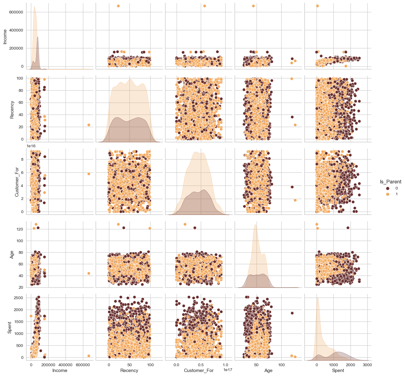
plt.show()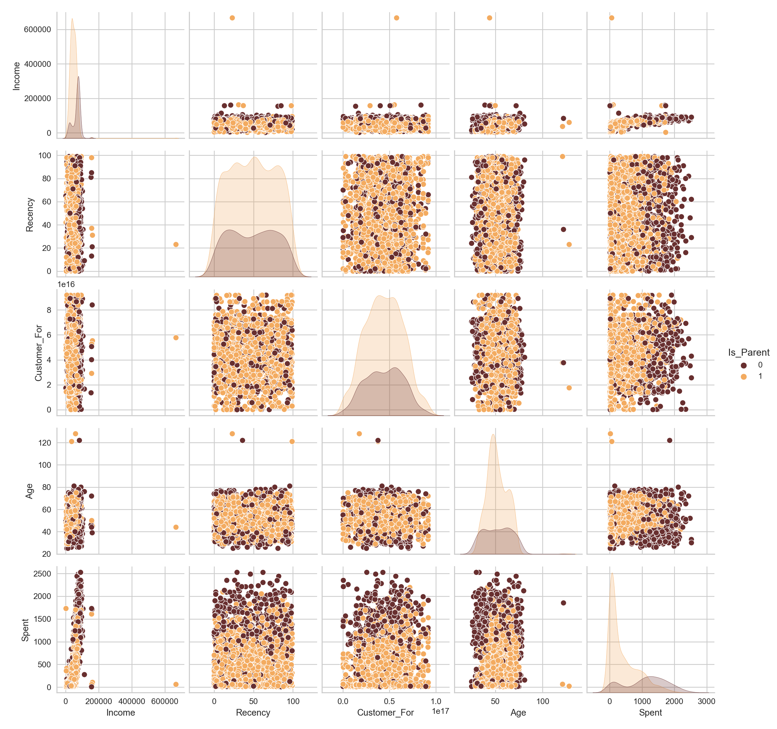
Clearly, there are a few outliers in the Income and Age features. I will be deleting the outliers in the data.
#Dropping the outliers by setting a cap on Age and income.
data = data[(data["Age"]<90)]
data = data[(data["Income"]<600000)]
print("The total number of data-points after removing the outliers are:", len(data))
The total number of data-points after removing the outliers are: 2212Next, let us look at the correlation amongst the features. (Excluding the categorical attributes at this point)
#correlation matrix
corrmat= data.corr()
sns.heatmap(corrmat,annot=True, center=0);
plt.show()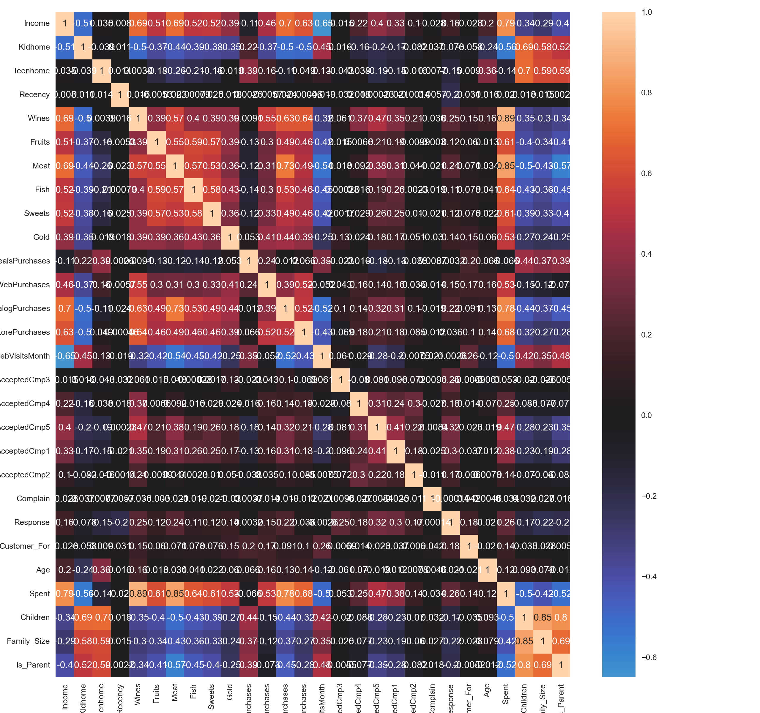
The data is quite clean and the new features have been included. I will proceed to the next step. That is, preprocessing the data.
Data Preprocessing
In this section, I will be preprocessing the data to perform clustering operations.
The following steps are applied to preprocess the data:
- Label encoding the categorical features
- Scaling the features using the standard scaler
- Creating a subset dataframe for dimensionality reduction
#Get list of categorical variables
s = (data.dtypes == 'object')
object_cols = list(s[s].index)

print("Categorical variables in the dataset:", object_cols)
Categorical variables in the dataset: ['Education', 'Living_With']#Label Encoding the object dtypes.
LE=LabelEncoder()
for i in object_cols:
data[i]=data[[i]].apply(LE.fit_transform)
print("All features are now numerical")All features are now numerical#Creating a copy of data
ds = data.copy()
# creating a subset of dataframe by dropping the features on deals accepted and promotions
cols_del = ['AcceptedCmp3', 'AcceptedCmp4', 'AcceptedCmp5', 'AcceptedCmp1','AcceptedCmp2', 'Complain', 'Response']
ds = ds.drop(cols_del, axis=1)
#Scaling
scaler = StandardScaler()
scaler.fit(ds)StandardScaler()scaled_ds = pd.DataFrame(scaler.transform(ds),columns= ds.columns )
print("All features are now scaled")All features are now scaled#Scaled data to be used for reducing the dimensionality
print("Dataframe to be used for further modelling:")Dataframe to be used for further modelling:
scaled_head=scaled_ds.head()
scaled_head.to_html()| Education | Income | Kidhome | Teenhome | Recency | Wines | Fruits | Meat | Fish | Sweets | Gold | NumDealsPurchases | NumWebPurchases | NumCatalogPurchases | NumStorePurchases | NumWebVisitsMonth | Customer_For | Age | Spent | Living_With | Children | Family_Size | Is_Parent | |
|---|---|---|---|---|---|---|---|---|---|---|---|---|---|---|---|---|---|---|---|---|---|---|---|
| 0 | -0.893586 | 0.287105 | -0.822754 | -0.929699 | 0.310353 | 0.977660 | 1.552041 | 1.690293 | 2.453472 | 1.483713 | 0.852576 | 0.351030 | 1.426865 | 2.503607 | -0.555814 | 0.692181 | 1.973583 | 1.018352 | 1.676245 | -1.349603 | -1.264598 | -1.758359 | -1.581139 |
| 1 | -0.893586 | -0.260882 | 1.040021 | 0.908097 | -0.380813 | -0.872618 | -0.637461 | -0.718230 | -0.651004 | -0.634019 | -0.733642 | -0.168701 | -1.126420 | -0.571340 | -1.171160 | -0.132545 | -1.665144 | 1.274785 | -0.963297 | -1.349603 | 1.404572 | 0.449070 | 0.632456 |
| 2 | -0.893586 | 0.913196 | -0.822754 | -0.929699 | -0.795514 | 0.357935 | 0.570540 | -0.178542 | 1.339513 | -0.147184 | -0.037254 | -0.688432 | 1.426865 | -0.229679 | 1.290224 | -0.544908 | -0.172664 | 0.334530 | 0.280110 | 0.740959 | -1.264598 | -0.654644 | -1.581139 |
| 3 | -0.893586 | -1.176114 | 1.040021 | -0.929699 | -0.795514 | -0.872618 | -0.561961 | -0.655787 | -0.504911 | -0.585335 | -0.752987 | -0.168701 | -0.761665 | -0.913000 | -0.555814 | 0.279818 | -1.923210 | -1.289547 | -0.920135 | 0.740959 | 0.069987 | 0.449070 | 0.632456 |
| 4 | 0.571657 | 0.294307 | 1.040021 | -0.929699 | 1.554453 | -0.392257 | 0.419540 | -0.218684 | 0.152508 | -0.001133 | -0.559545 | 1.390492 | 0.332600 | 0.111982 | 0.059532 | -0.132545 | -0.822130 | -1.033114 | -0.307562 | 0.740959 | 0.069987 | 0.449070 | 0.632456 |
’
Dimensionality Reduction
In this problem, there are many factors on the basis of which the final classification will be done. These factors are basically attributes or features. The higher the number of features, the harder it is to work with it. Many of these features are correlated, and hence redundant. This is why I will be performing dimensionality reduction on the selected features before putting them through a classifier. Dimensionality reduction is the process of reducing the number of random variables under consideration, by obtaining a set of principal variables.
Principal component analysis (PCA) is a technique for reducing the dimensionality of such datasets, increasing interpretability but at the same time minimizing information loss.
Steps in this section:
- Dimensionality reduction with PCA
- Plotting the reduced dataframe
Dimensionality reduction with PCA
For this project, I will be reducing the dimensions to 3.
#Initiating PCA to reduce dimentions aka features to 3
pca = PCA(n_components=3)
pca.fit(scaled_ds)
PCA(n_components=3)
PCA_ds = pd.DataFrame(pca.transform(scaled_ds), columns=(["col1","col2", "col3"]))
pca_t=PCA_ds.describe().T
pca_t.to_html()| count | mean | std | min | 25% | 50% | 75% | max | |
|---|---|---|---|---|---|---|---|---|
| col1 | 2212.0 | -1.284887e-17 | 2.878377 | -5.969394 | -2.538494 | -0.780421 | 2.383290 | 7.444305 |
| col2 | 2212.0 | 3.212219e-17 | 1.706839 | -4.312196 | -1.328316 | -0.158123 | 1.242289 | 6.142721 |
| col3 | 2212.0 | 7.307797e-17 | 1.221956 | -3.530416 | -0.829067 | -0.022692 | 0.799895 | 6.611222 |
’
#A 3D Projection Of Data In The Reduced Dimension
x =PCA_ds["col1"]
y =PCA_ds["col2"]
z =PCA_ds["col3"]
#To plot
fig = plt.figure(figsize=(10,8))
ax = fig.add_subplot(111, projection="3d")
ax.scatter(x,y,z, c="maroon", marker="o" )
ax.set_title("A 3D Projection Of Data In The Reduced Dimension")
plt.show()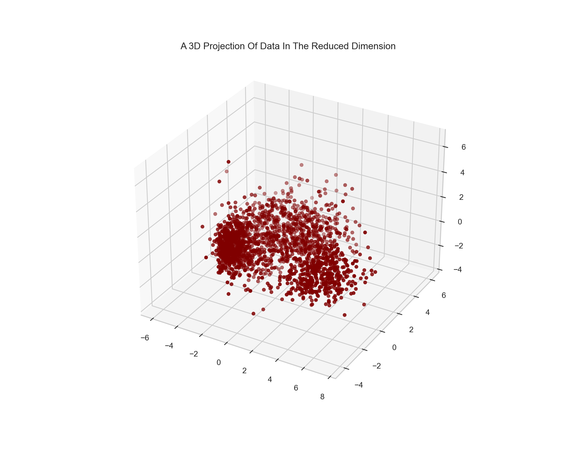
Clustering
Now that I have reduced the attributes to three dimensions, I will be performing clustering via Agglomerative clustering. Agglomerative clustering is a hierarchical clustering method. It involves merging examples until the desired number of clusters is achieved.
Steps involved in the Clustering
- Clustering via Agglomerative Clustering
- Examining the clusters formed via scatter plot
#Initiating the Agglomerative Clustering model
AC = AgglomerativeClustering(n_clusters=4)
# fit model and predict clusters
yhat_AC = AC.fit_predict(PCA_ds)
PCA_ds["Clusters"] = yhat_AC
#Adding the Clusters feature to the orignal dataframe.
data["Clusters"]= yhat_AC
To examine the clusters formed let’s have a look at the 3-D distribution of the clusters.
#Plotting the clusters
fig = plt.figure(figsize=(10,8))
ax = plt.subplot(111, projection='3d', label="bla")
ax.scatter(x, y, z, s=40, c=PCA_ds["Clusters"], marker='o')
ax.set_title("The Plot Of The Clusters")
plt.show()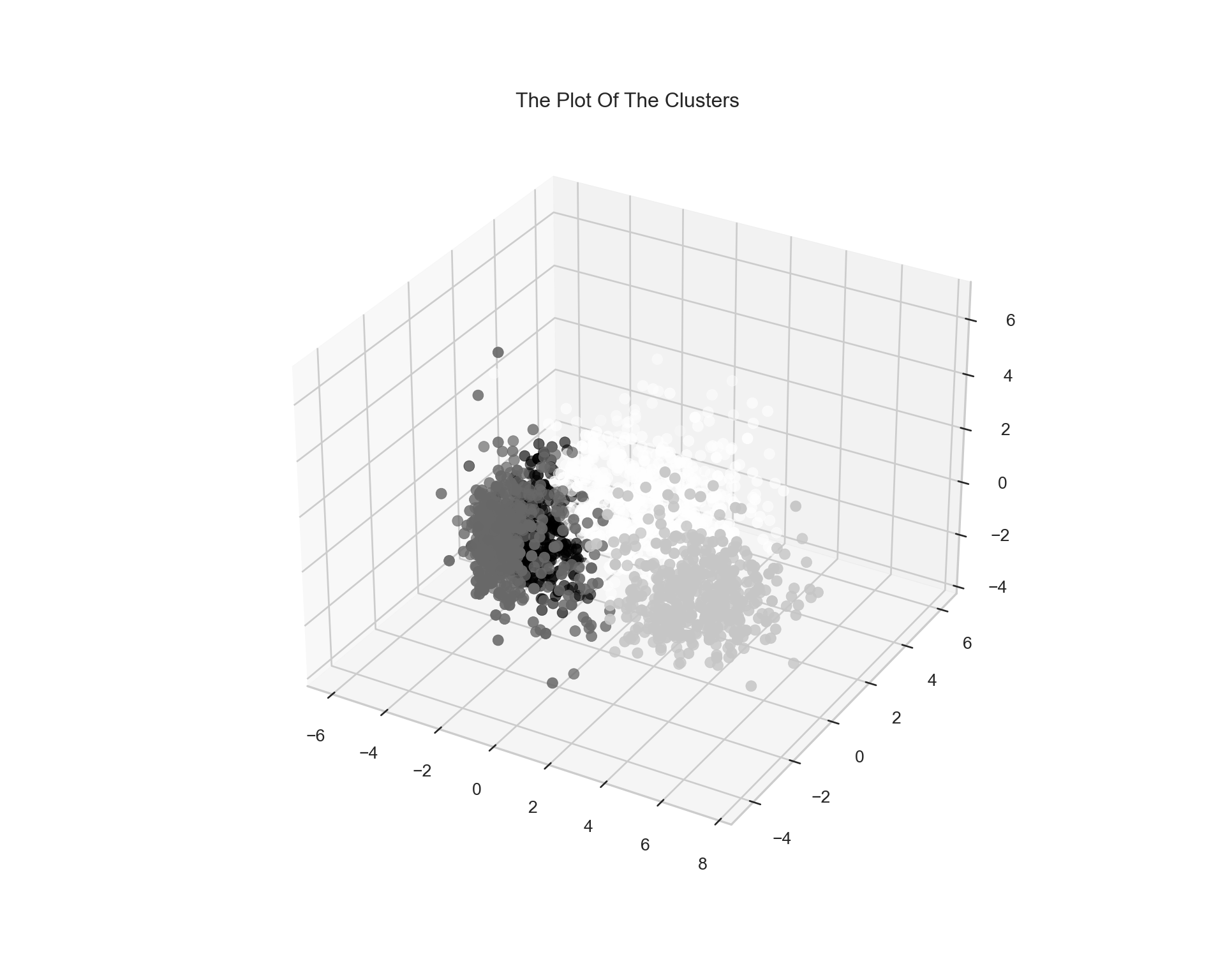
Evaluating Models
Since this is an unsupervised clustering. We do not have a tagged feature to evaluate or score our model. The purpose of this section is to study the patterns in the clusters formed and determine the nature of the clusters’ patterns.
For that, we will be having a look at the data in light of clusters via exploratory data analysis and drawing conclusions.
Firstly, let us have a look at the group distribution of clustring
#Plotting countplot of clusters
pal = ["#682F2F","#B9C0C9", "#9F8A78","#F3AB60"]
pl = sns.countplot(x=data["Clusters"], palette= pal);
pl.set_title("Distribution Of The Clusters");
plt.show()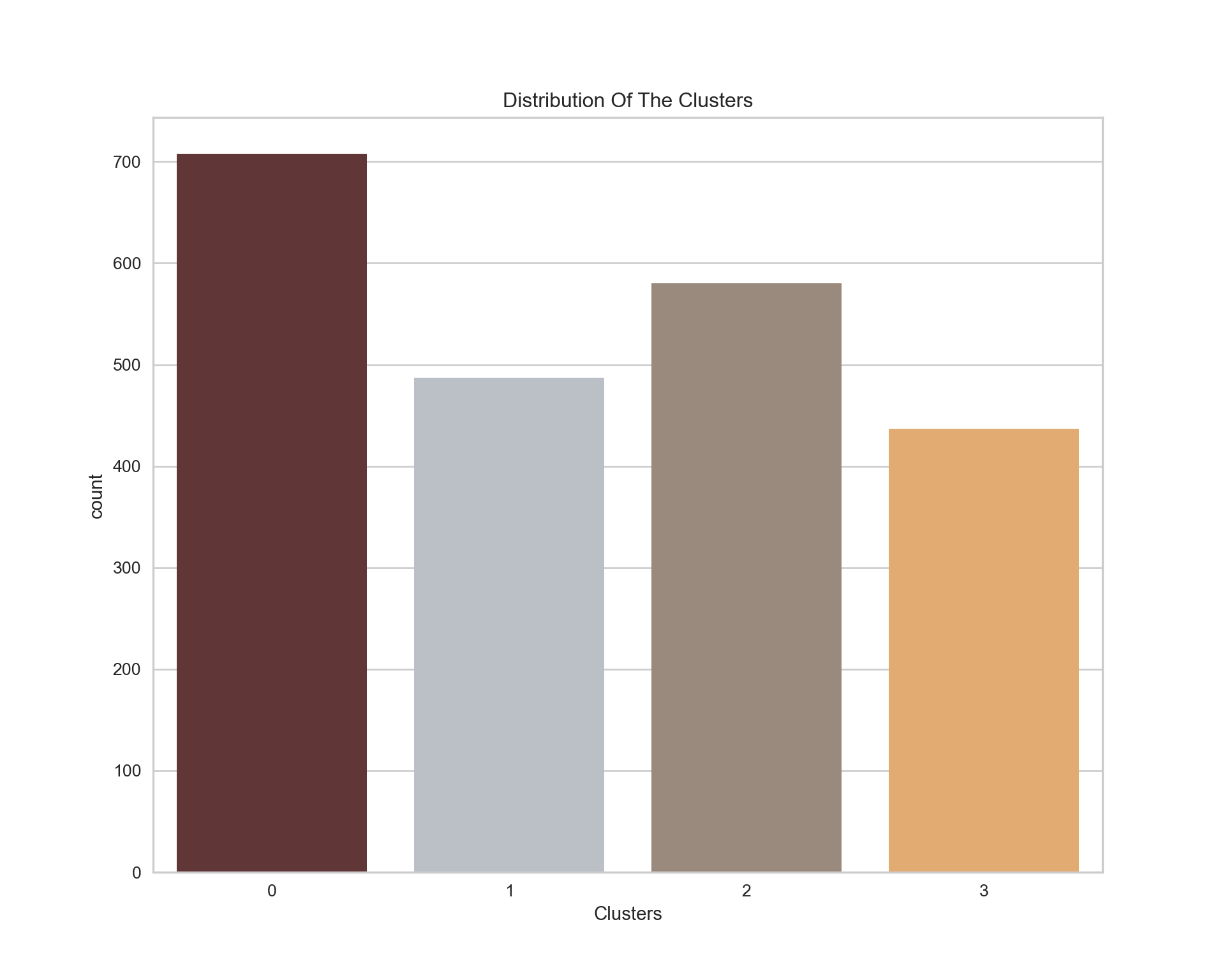
The clusters seem to be fairly distributed.
pl = sns.scatterplot(data = data,x=data["Spent"], y=data["Income"],hue=data["Clusters"], palette= pal)
pl.set_title("Cluster's Profile Based On Income And Spending");
plt.legend();
plt.show()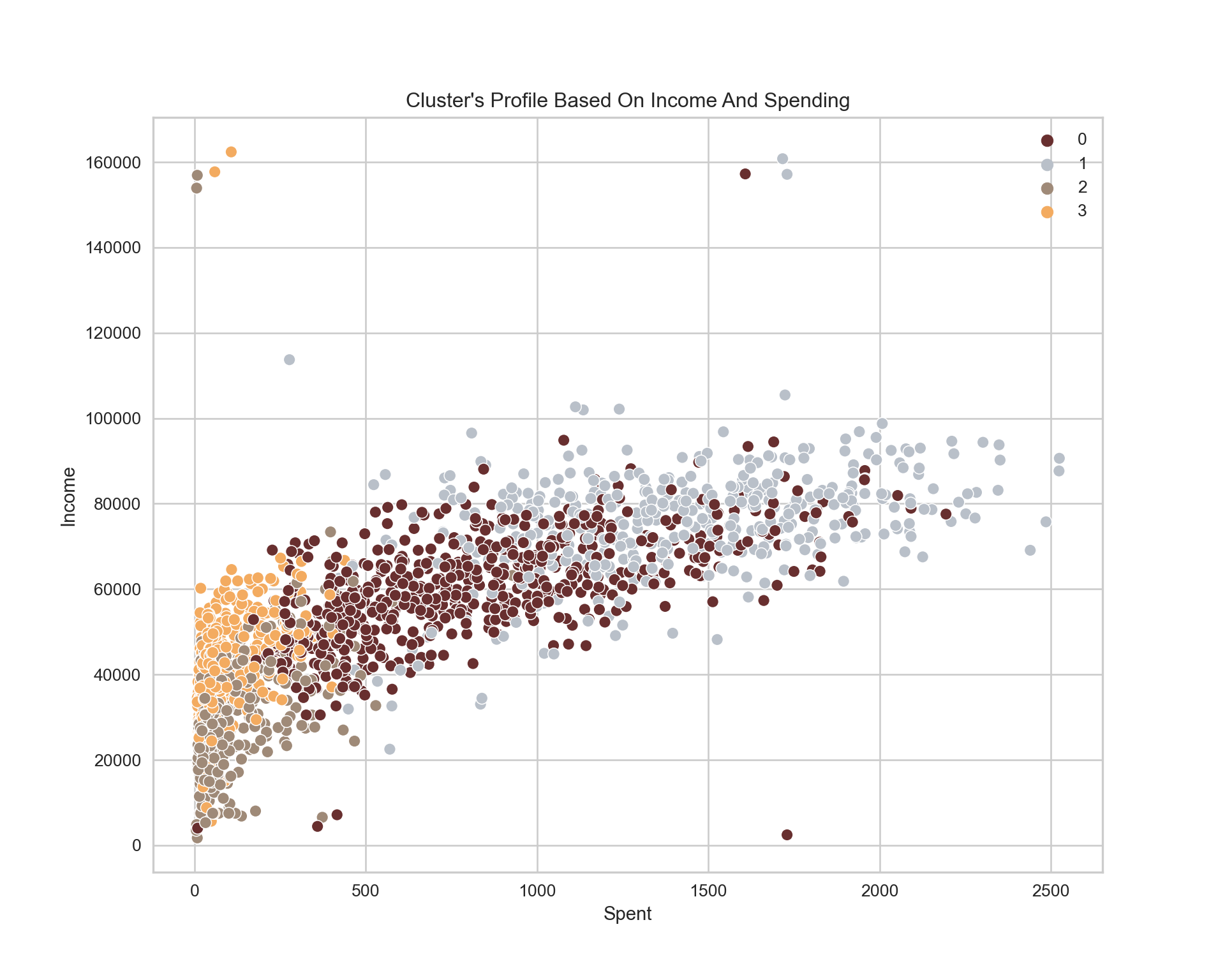
Income vs spending plot shows the clusters pattern
- Group 0: high spending & average income
- Group 1: high spending & high income
- Group 2: low spending & low income
- Group 3: high spending & low income
Next, I will be looking at the detailed distribution of clusters as per the various products in the data. Namely: Wines, Fruits, Meat, Fish, Sweets and Gold
plt.figure()
pl=sns.swarmplot(x=data["Clusters"], y=data["Spent"], color= "#CBEDDD", alpha=0.5 )
pl=sns.boxenplot(x=data["Clusters"], y=data["Spent"], palette=pal)
plt.show()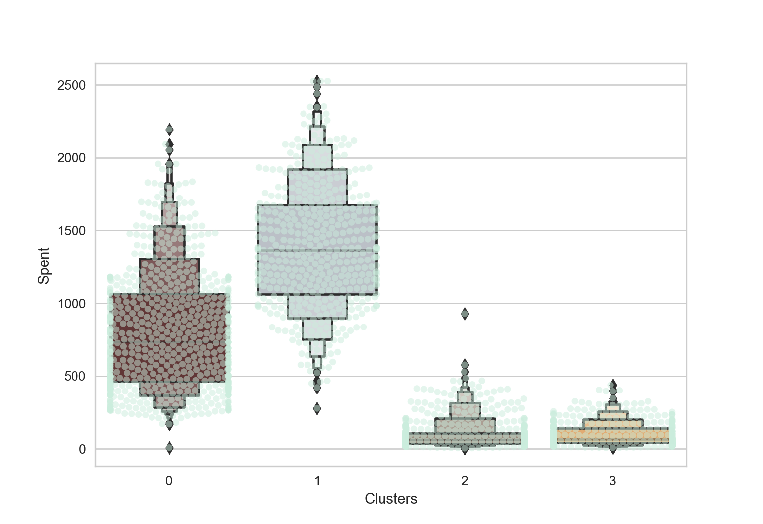
From the above plot, it can be clearly seen that cluster 1 is our biggest set of customers closely followed by cluster 0. We can explore what each cluster is spending on for the targeted marketing strategies.
Let us next explore how did our campaigns do in the past.
#Creating a feature to get a sum of accepted promotions
data["Total_Promos"] = data["AcceptedCmp1"]+ data["AcceptedCmp2"]+ data["AcceptedCmp3"]+ data["AcceptedCmp4"]+ data["AcceptedCmp5"]
#Plotting count of total campaign accepted.
plt.figure()
pl = sns.countplot(x=data["Total_Promos"],hue=data["Clusters"], palette= pal)
pl.set_title("Count Of Promotion Accepted")
pl.set_xlabel("Number Of Total Accepted Promotions")
plt.show()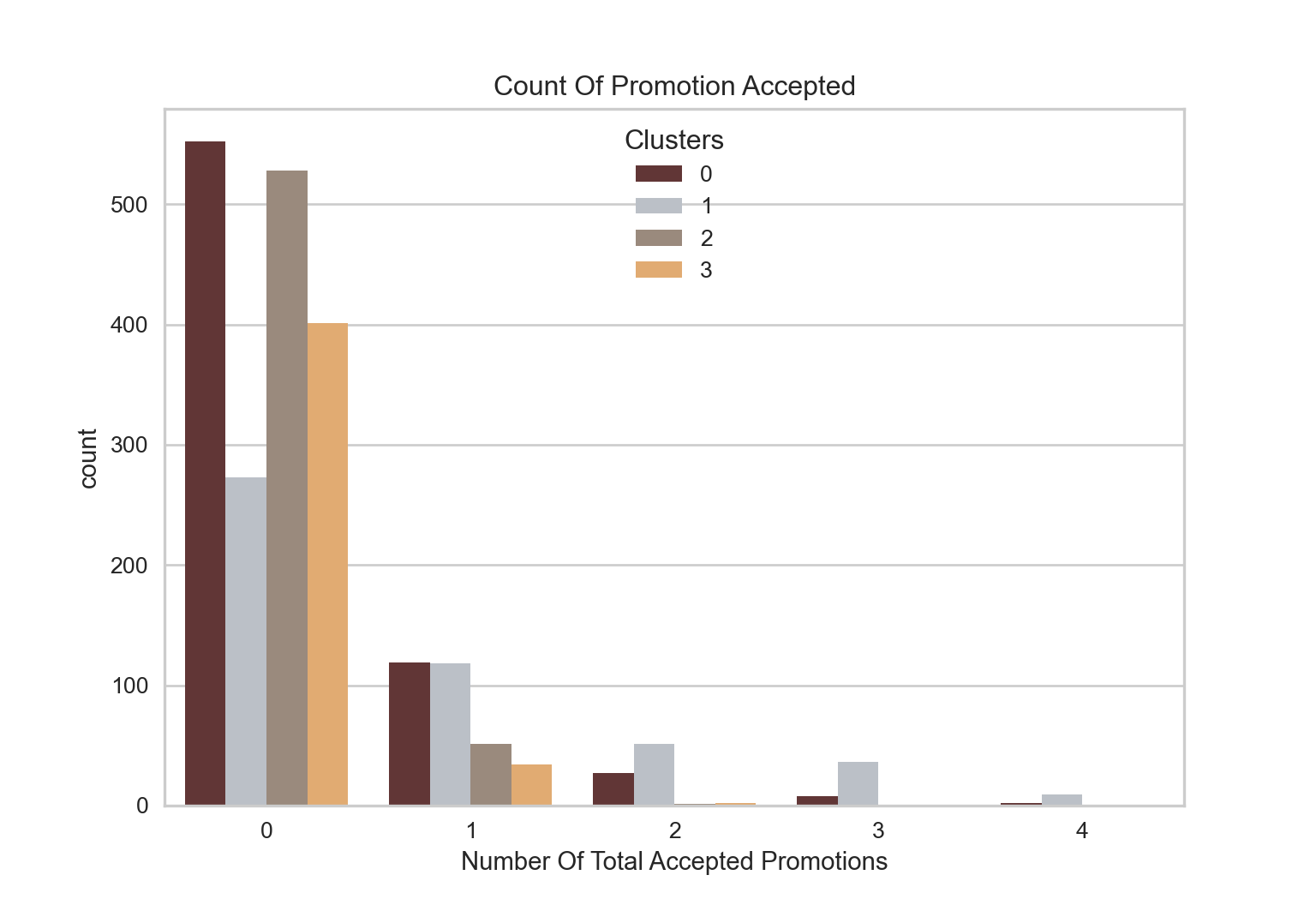
There has not been an overwhelming response to the campaigns so far. Very few participants overall. Moreover, no one part take in all 5 of them. Perhaps better-targeted and well-planned campaigns are required to boost sales.
#Plotting the number of deals purchased
plt.figure()
pl=sns.boxenplot(y=data["NumDealsPurchases"],x=data["Clusters"], palette= pal)
pl.set_title("Number of Deals Purchased")
plt.show()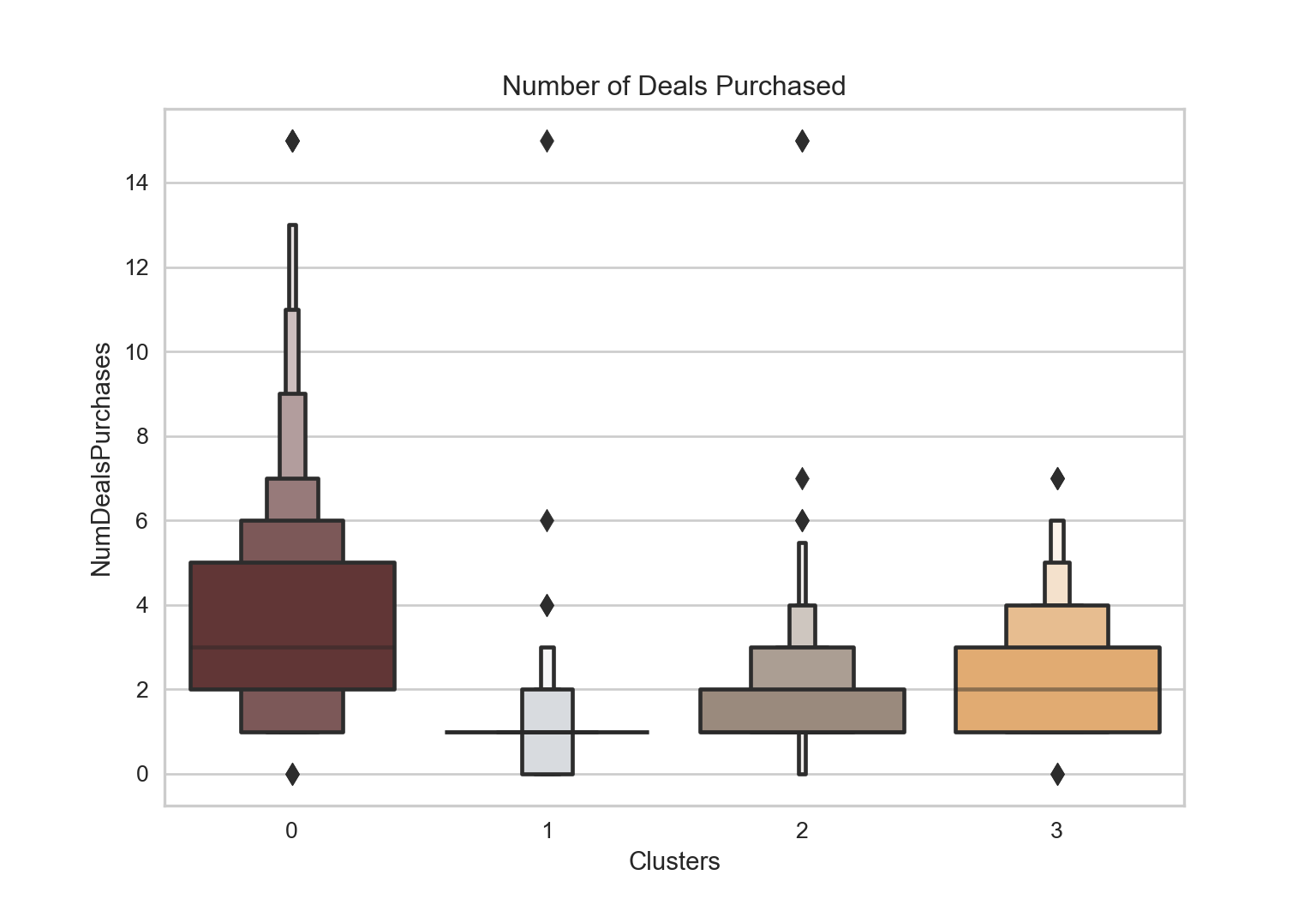
Unlike campaigns, the deals offered did well. It has best outcome with cluster 0 and cluster 3. However, our star customers cluster 1 are not much into the deals. Nothing seems to attract cluster 2 overwhelmingly
Profiling
Now that we have formed the clusters and looked at their purchasing habits. Let us see who all are there in these clusters. For that, we will be profiling the clusters formed and come to a conclusion about who is our star customer and who needs more attention from the retail store’s marketing team.
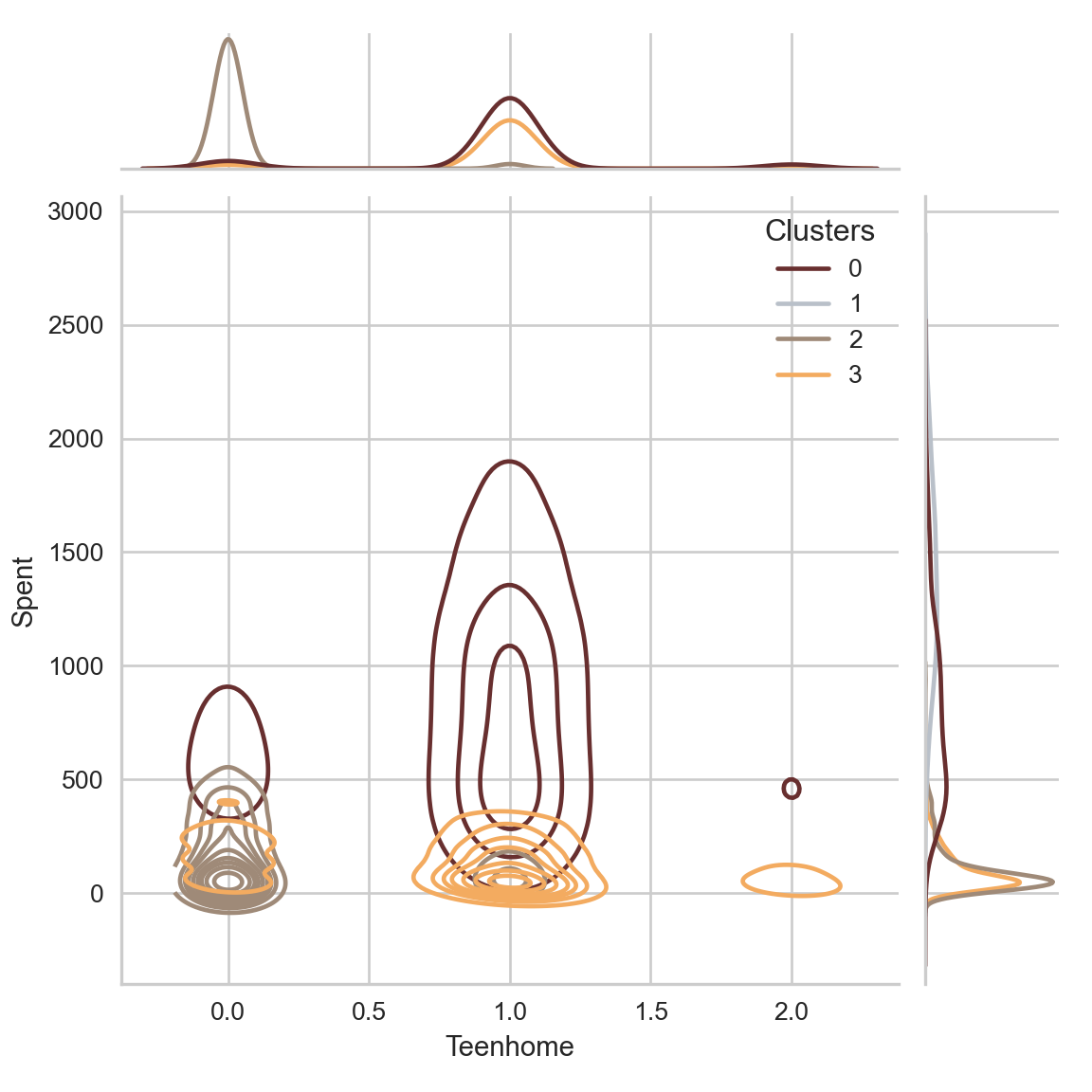
To decide that I will be plotting some of the features that are indicative of the customer’s personal traits in light of the cluster they are in. On the basis of the outcomes, I will be arriving at the conclusions.
Personal = [ "Kidhome","Teenhome","Customer_For", "Age", "Children", "Family_Size", "Is_Parent", "Education","Living_With"]

for i in Personal:
    plt.figure();
    sns.jointplot(x=data[i], y=data["Spent"], hue =data["Clusters"], kind="kde", palette=pal);
    plt.show()
<Figure size 800x550 with 0 Axes>
<seaborn.axisgrid.JointGrid object at 0x0000000055B103D0>
<Figure size 800x550 with 0 Axes>
<seaborn.axisgrid.JointGrid object at 0x00000000562DB0D0>
<Figure size 800x550 with 0 Axes>
<seaborn.axisgrid.JointGrid object at 0x000000005639FC40>
<Figure size 800x550 with 0 Axes>
<seaborn.axisgrid.JointGrid object at 0x000000005563B580>
<Figure size 800x550 with 0 Axes>
<seaborn.axisgrid.JointGrid object at 0x00000000557B5550>
<Figure size 800x550 with 0 Axes>
<seaborn.axisgrid.JointGrid object at 0x0000000055A2B100>
<Figure size 800x550 with 0 Axes>
<seaborn.axisgrid.JointGrid object at 0x00000000562F0550>
<Figure size 800x550 with 0 Axes>
<seaborn.axisgrid.JointGrid object at 0x0000000055841880>
<Figure size 800x550 with 0 Axes>
<seaborn.axisgrid.JointGrid object at 0x000000005454AD90>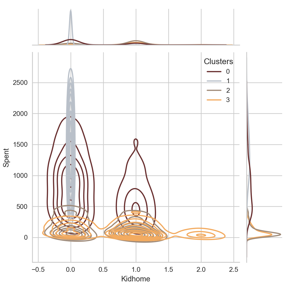
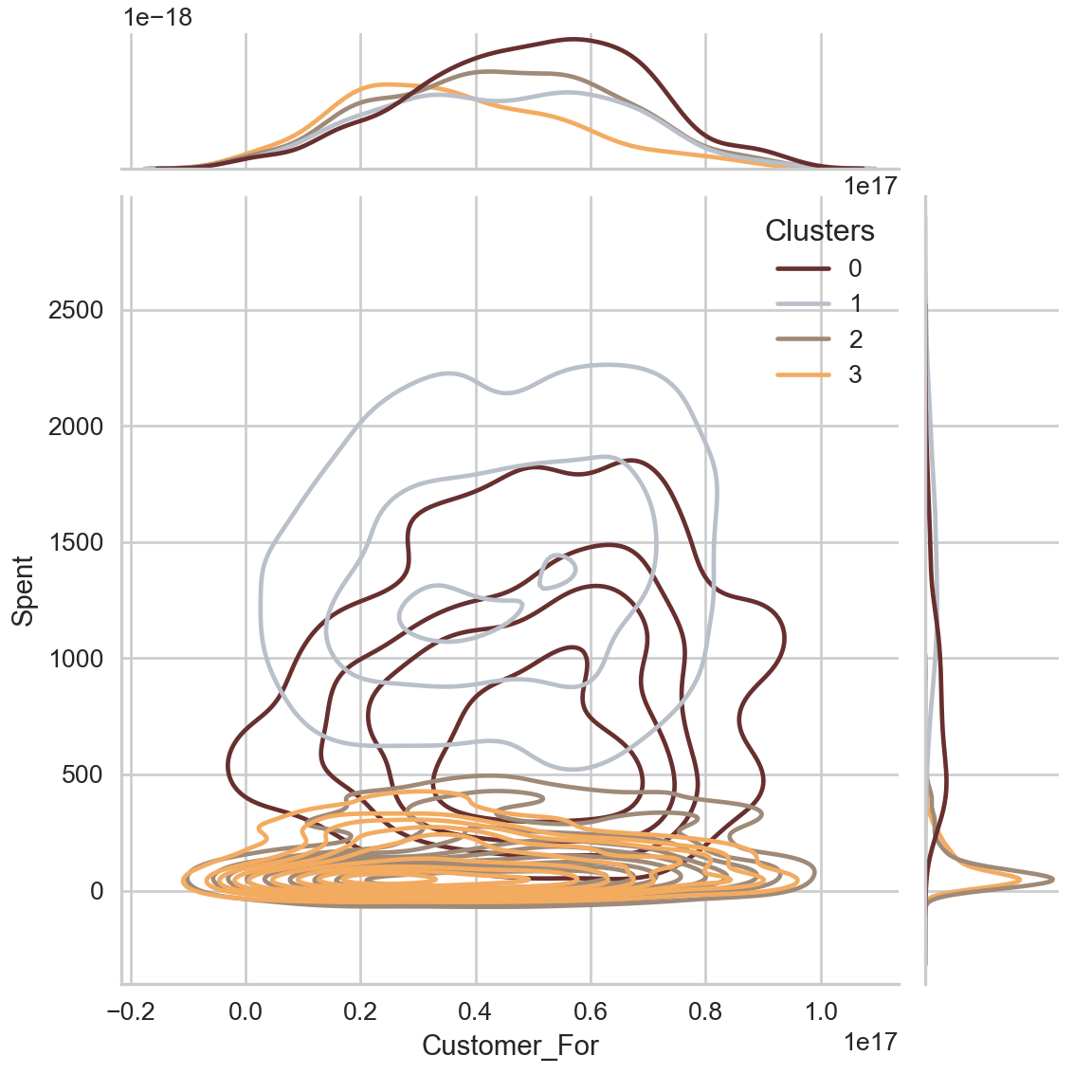
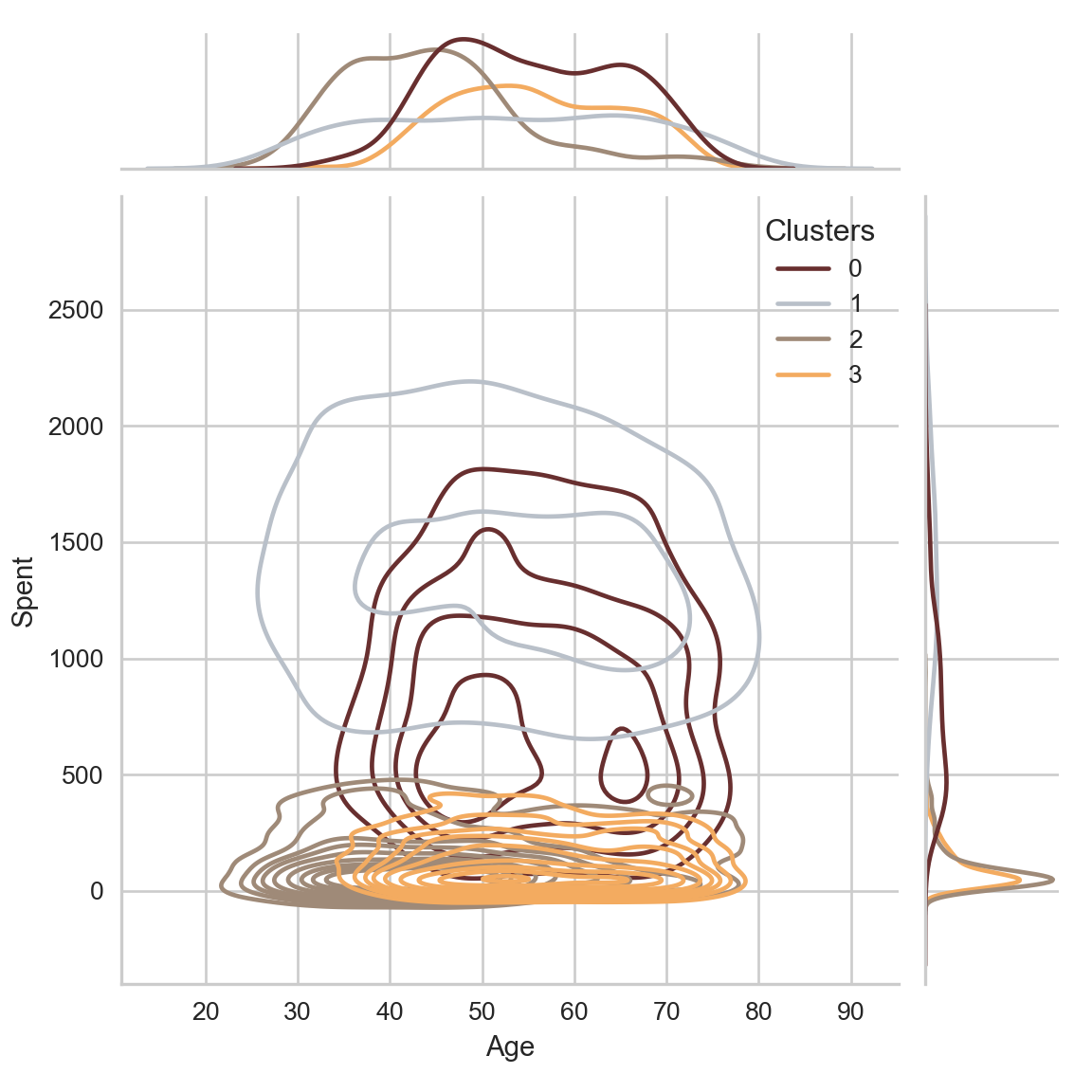
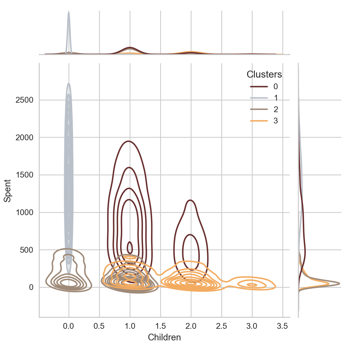
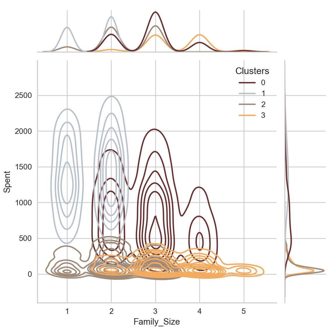
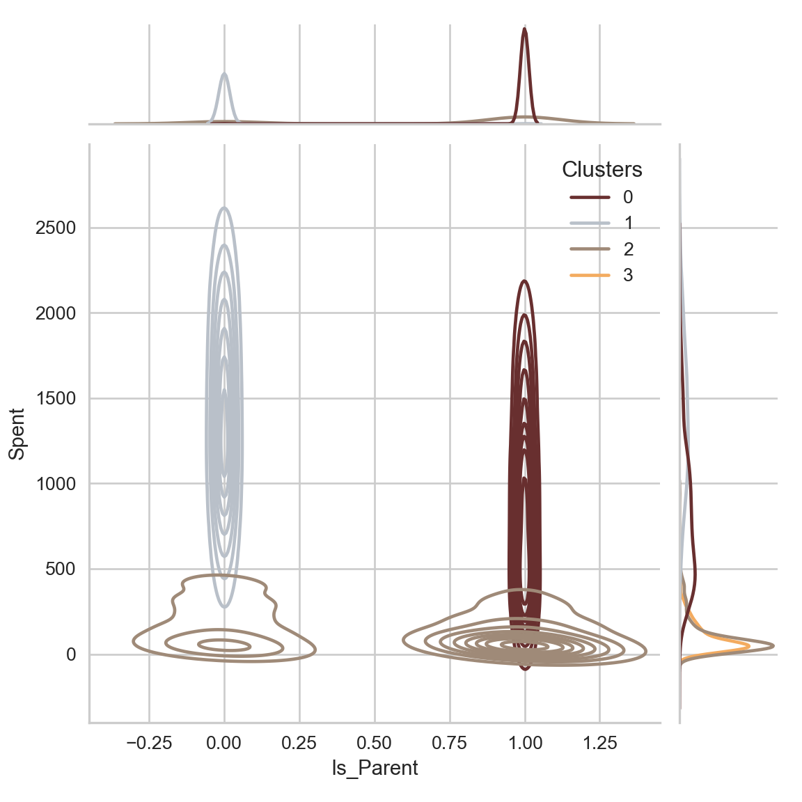
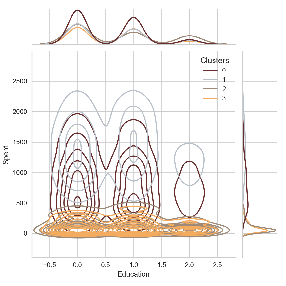
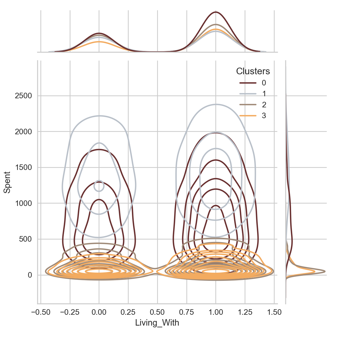
Points to be noted:
- About Cluster Number 0:
- Are a definitely a parent
- At the max have 4 member in the family and at least 2
- Single Parents are a subset of this group
- Relatively older
- About Cluster Number 1:
- Are a definitely not a parent
- At the max have 2 member in the family
- A slight majority of couples over single people
- Span all ages
- A high income group
- About Cluster Number 2:
- The majority of these people are parents
- At the max are 3 members in the family
- The majority have one kid (and not teenagers, typically)
- Relatively younger
- About Cluster Number 3:
- Are a definitely not a parent
- At the max have 5 member in the family and at least 2
- The majority have teenagers at home
- Relatively older
- A lower-income group
Conclusion
In this project, I performed unsupervised clustering. I did use dimensionality reduction followed by agglomerative clustering. I came up with 4 clusters and further used them in profiling customers in clusters according to their family structures and income/spending. This can be used in planning better marketing strategies.